In this post I'll use elements from local theory of curves and surfaces to arrive at Gauss's remarkable theorem ("Theorema Egregium") and highlight the significance of the distinction between intrinsic and extrinisic properties of a surface. Everything should be comprehensible if one has a background in multivariable vector calculus and linear algebra, and maybe basic topology.

Curvature

We define the curvature of a curve $\alpha$, parameterized by arc length, to be $$\kappa(s) = \| \alpha'' \|.$$
This makes sense because it measures the rate of change of the tangent of $\alpha$, thus being a metric for how much the curve curves.

Now, we define the unit tangent vector of $\alpha$ at $s$ as $T(s) = \alpha'(s)$, the principal normal vector as $N(s) = T'(s)\left.\right/\|T'(s)\|$ and the binormal vector as $B(s) = T(s) \times N(s)$ . The vectors $\{T, N, B\}$, together called a Frenet frame, are orthonormal and form a basis for $\mathbb{R}^3$

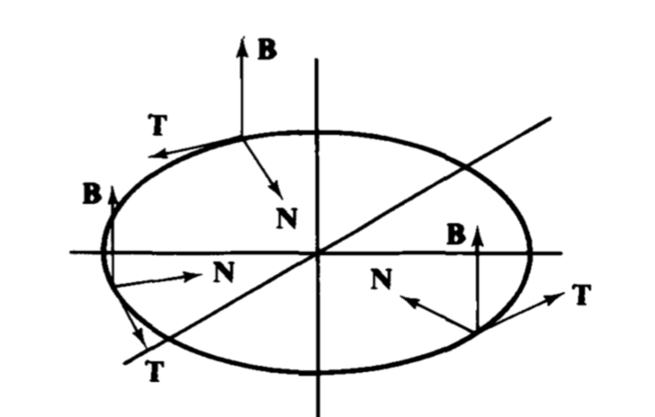
Note: $T'(s) = \alpha''(s) = \kappa N(s)$.

We'll work with "surfaces" as coordinate patches, though all of this extensible and applicable onto general manifolds.
Consider a unit speed curve $\gamma$ on a surface $M$ parameterized as $x: U \to \mathbb{R}^3$ for open $U \subset \mathbb{R}^2$. There must exist $C^k$ curves $\gamma^1, \gamma^2$ such that $$\gamma(s) = x(\gamma^1(s), \gamma^2(s)).$$
Then, let $n$ be the unit normal to the surface and $n(t) = n \circ \gamma(t)$ be the restriction of $n$ on $\gamma$. We call $S = n \times T$ the intrinsic normal of $\gamma$ on the surface. If $U$ has coordinates $u^1$ and $u^2$, by the chain rule we have $$T = \gamma' = \sum \frac{\partial x}{\partial u^i} (\gamma ^i)'.$$

Notation: $x_i = \frac{\partial x}{\partial u^i} $. Then, we have $$\gamma'(s) = \sum x_i(\gamma^1(s), \gamma^2(s))(\gamma^i(s))'$$
and $$\gamma'' = \sum_{i, j} x_{ij} (\gamma^i)' (\gamma^j)' + \sum x_i (\gamma^i)''.$$
Now let $P$ be any point on the surface $M$. Then, $T_PM$, the tangent space, is the set of all vectors tangent to $M$ at $P$, while $N_PM$, the normal space, is the set of vectors perpendicular to $M$ at $P$. Clearly $T_PM + N_PM = \mathbb{R}^3$. Thus, any vector can be represented as a linear combination of a vector in $T_PM$ and a vector in $N_PM$. In particular, this can be done for $\gamma''$. Thus we have $$\gamma''(s) = C(s) + D(s)$$ where $C(s)$ is tangent to $M$ and $D(s)$ is normal to $M$.

Then, since $T$ is tangent to $M$, $\left< D, T \right> = 0$. Also, $\left< \gamma'', T\right> = 0$, and thus $\left< C, T\right> = 0$. This means $C$ is a perpendicular to both $n$ and $T$, and thus is a multiple of $S = n \times T$. Then we can define the normal curvature $\kappa_n(s)$ and the geodesic curvature $\kappa_g(s)$ as $$\kappa(s) N(s) = \gamma'' = \kappa_n(s)n(s) + \kappa_g(s) S(s).$$This also gives us that $$\kappa^2 = \kappa_n^2 + \kappa_g ^2.$$

First and second form

We introduce the concept of forms because they help us generalize the notion of lengths and areas on surfaces (they are called “forms” to indicate that they are bilinear in the linear algebra sense). We define the first form $I : T_PM \times T_PM \to \mathbb{R}$ as $I(X, Y) = \left< X, Y\right>$. That is, for vectors $X = \sum X^i x_i$ and $Y = \sum Y^i y_i$ on the tangent place of a surface $M$ at point $P$, we have $$I(X, Y) = \left< X, Y\right> = \sum_{i, j} X^iY^j\left< x_i, x_j\right>.$$
Notation: $g_{ij}(u^1, u^2) = \left< x_i(u^1, u^2), x_j(u^1, u^2)\right>$, or $g_{ij} = \left< x_1, x_2 \right>$, where $u^i$ are the coordinates for $U$.
Then we have $$I(X, Y) = \sum_{i, j}X^iY^jg_{ij}.$$
The $g_{ij}$ are called the coefficients of the metric tensor. The term “metric” is used to denote that the $g_{ij}$ can be used to calculate measures of different orders. For example, if $\alpha(s)$ is a curve on the surface $M$ which has the embedding $x: U \to \mathbb{R}^3$, we have $\alpha(s) = x(\alpha^1(s), \alpha^2(s))$. Then, the length of the curve $\alpha: [a, b] \to \mathbb{R}^3$ is given by $$\int_a^b \left | \frac{d \alpha}{dt} \right| dt$$
but $\frac{d \alpha}{dt} = \sum x_i (\alpha^i)'$ and so
\begin{align} \left| \frac{d \alpha}{dt} \right| &= \sqrt{\left< \frac{d \alpha}{dt}, \frac{d \alpha}{dt} \right>}\\ &= \sqrt{\left< \sum x_i (\alpha^i)', \sum x_j (\alpha^j)' \right>}\\ &= \sqrt{\sum g_{ij} (\alpha^i)' (\alpha^j)'} \end{align} and the length of the curve is $$\int_a^b \sqrt{\sum g_{ij} (\alpha^i)' (\alpha^j)' dt}.$$
Notation: $g = \det(g_{ij})$ and $g^{kl} = (k, l)$ entry of the inverse matrix of $(g_{ij})$

Lemma. For a surface $x: U \to \mathbb{R}^3$ the following hold:
a) $g = \left| x_1 \times x_2 \right|^2$
b) $g^{11} = g_{22}/g, g^{12} = g^{21} = -g_{12}/g, g^{22} = g_{11}/g$
c) $\forall i, j, \sum_k g_{ik}g^{kj} = \delta_i^j$, where $\delta_i^j$ are the $(i, j)$th entries of the identity matrix.

In the way we had defined the first fundamental form as $I(X, Y) = \sum_{i, j}X^iY^jg_{ij}$, we define the second fundamental form as $$II(X, Y) = \sum_{i, j} X^i, Y^j L_{ij}$$
where we define $L_{ij}$, the coefficients of the second fundamental form, to be $$L_{ij} = \langle x_{ij}, n\rangle.$$
Viewing the second form as a generalization of length we can ask which vectors have “generalized length” $\pm 1$ with respect to $II$. This gives rise to the Dupin indicatrix, which gives information about the geometry of $M$ near $P$, but I will not digress into that here further.
Notation: we define the Christoffel symbols $\Gamma_{ij}^{k}$ on $U$ as $\Gamma_{ij}^{k} = \sum_{l}\langle x_{ij}, x_l \rangle g^{lk}.$
We introduce the Christoffel symbols because they lead to this remarkable formula, courtesy of Gauss, that $L_{ij}$ measures the normal component of $x_{ij}$ while $\Gamma_{ij}^{k}$ measure the tangential component of $x_{ij}$. In other words, $$x_{ij} = L_{ij} n + \sum_k \Gamma_{ij}^k x_k.$$

Using Gauss' formula we also get that for a curve $\gamma$ on $x$, $$\kappa_n = \sum_{ij} L_{ij} (\gamma^i)' (\gamma^j)'$$
and
$$\kappa_g S = \sum_{k} \left[ (\gamma^{ii})' + \sum_{ij} \Gamma_{ij}^k (\gamma^i)' (\gamma^j)'\right]x_k.$$ It took me a while to understand why we even introduce the metric tensor, since we were arriving at it using the surface embedding in the first place. It seemed like it was just notational jargon asbtracting away a very simple and clear picture. It finally made sense when I saw that you can actually define the metric tensor on a surface without describing the embedding, and that itself allows you to compute a lot of properties of the surface, such as length of curves of the surface and curvatures. It's why we make the distinction in defining a symbol as being intrinsic or extrinsic, since those expressions that are intrinsic don't require us to know about the particular parameterization of the surface––we can just work with the metric tensor.

For example, the Christoffel symbols, which so apparently seem to depend on the surface's parameterization in their definition are actually an intrinsic property of the surface. In particular, we have $$\Gamma_{ij}^k = \dfrac{1}{2}\sum_{k = 1}^2g^{kl}\left(\ \dfrac{\partial g_{ik}}{\partial u_j} - \dfrac{\partial g_{ik}}{\partial u_j} + \dfrac{\partial g_{ik}}{\partial u_j} \right).$$
The geodesic curvature, $\kappa_g$, too is intrinsic. This means that two-dimensional beings on a surface would be able calculate the lengths and angles, and thus the metric tensor, and be able to compute the geodesic curvature without any global knowledge of the surface they were on.

Theorema Egregium

We shall now discuss the construction of the Weingarten map (also called the shape operator) in preparation for defining the principal, mean, and Gaussian curvatures.

The Weingarten map $L$ is, for each $P \in M$, the function $L : T_PM \to \mathbb{R}^3$ given by $X \mapsto -\nabla_X n(P)$, which describes the normal curvature of $M$ at $P$ in the direction of $X$. The $-$ is just for convenience.

Now, with respect to coordinates $u^1$ and $u^2$, the matrix $L$ is given by $(g^{kl})(L_{ij})$. Note that $L$ is self-adjoint and hence has real eigenvalues, which are the roots of the equation $$0 = \det(L - \lambda I).$$ We denote these roots $\kappa_1$ and $\kappa_2$, which will be called the principal curvatures of $M$ at $P$. Then, the mean curvature $H$ is simply $\dfrac{\kappa_1 + \kappa_2}{2}$ and the Gaussian curvature, K, $\kappa_1\kappa_2$.

The Reimannian curvature tensor with indices $(i, j, k, l)$ is defined as $$R^l_{ijk} = \dfrac{\partial \Gamma_{ik}^l}{\partial u^j} - \dfrac{\partial \Gamma_{ij}^l}{\partial u^k} + \sum_p \left( \Gamma_{ik}^p \Gamma_{pj}^l - \Gamma_{ij}^p \Gamma_{pk}^l\right)$$
Note that the Reimannian curvature tensor is defined intrinsically. Seeing so many indices and differentials and summations, the geometric picture behind a lot of these symbols is often lost. However, there is a geometric intuition for the Reimannian curvature tensor, namely that taking parital derivatives on a surface is commutative if and only if the Reimannian curvature tensor on the surface is 0. In more general terms, it measures the degree to which the surface is locally isometric to the Euclidean space.

Gauss' equations. $R^l_{ijk} = L_{ik} L^l_j - L_{ij} L^l_k$, where $L^l_k = \sum L_{ik}g^{il}$ is the $(l, k)$th entry of the matrix of the Weingarten map.
With all this machinery, we are finally ready to prove Gauss' Theorema Egregium.

Theorem. The Gaussian curvature $K$ of a surface is intrinsic.
Proof. By Gauss' equation, $R^l_{ijk} = L_{ik} L^l_j - L_{ij} L^l_k$. Then,
$$\sum R^l_{ijk} g_{lm} = L_{ik}L_{mj} - L_{ij}L_{mk}$$ Now, let $i = k = 1$, and $j = m = 2$. Then,
\begin{align} \sum R^l_{121} g_{12} &= L_{11}L_{22} - L_{12}L_{21}\\ &= \det(L_{ij})\\ &= \det((L^k_j)(g_{ik}))\\ &= \det((L^k_j)) \det((g_{ik})) = Kg \end{align} Hence, we are done. $\blacksquare$